0.信息熵
计算公式
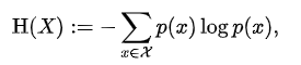
说明
Onehot向量的信息熵为0
非Onehot向量的概率分布反而有一定的信息熵
对于交叉熵而言,与Onehot向量相同的概率分布时,其交叉熵也为0
1.交叉熵损失 Cross Entropy Loss (CE loss)
计算公式:
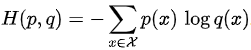
公式实际应用说明:
其中p(x)代表了标签(或者每个标签的概率),q(x)代表了模型预测的概率
代码示例
import torch
import torch.nn as nn
import torch.nn.functional as F
# logits shape: [BS, NC]
batchsize = 2
num_class = 4
# 神经网络的输出值,没有经过softmax,未归一化
logits = torch.randn(batchsize, num_class)
# delta 目标分布
hard_label = torch.randint(num_class, size=(batchsize,))
# 非 delta 目标分布
soft_label = torch.randn(batchsize, num_class)
### method 1 for CE loss
### hard label,常用在分类之中
ce_loss_fun = torch.nn.CrossEntropyLoss()
ce_loss = ce_loss_fun(logits, hard_label)
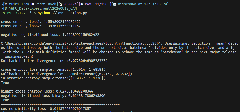
print(f"cross entropy loss1: {ce_loss}")
### method 2 for CE loss
### soft label,常用在知识蒸馏中
ce_loss = ce_loss_fun(logits, torch.softmax(soft_label, -1))
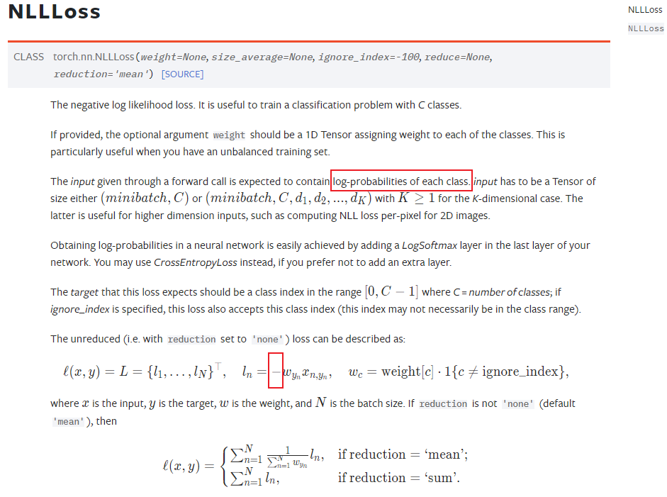
print(f"cross entropy loss2: {ce_loss}")2.负对数似然损失 Negative Log Likelihood Loss (NLL loss)
import torch
import torch.nn as nn
import torch.nn.functional as F

# logits shape: [BS, NC]
batchsize = 2
num_class = 4

# 神经网络的输出值,没有经过softmax,未归一化
logits = torch.randn(batchsize, num_class)
# delta 目标分布
hard_label = torch.randint(num_class, size=(batchsize,))

nll_fn = torch.nn.NLLLoss()
nll_loss = nll_fn(torch.log(torch.softmax(logits, dim=-1)), hard_label)  # 与 CE loss结果相同
print(f"negative log-likelihood loss: {nll_loss}")
### cross entropy value = NLL value
这里注意到:cross entropy value = NLL value
也就是说,能用CE loss的地方,就能用NLL loss
取决于输出的是什么,分两种情况:
- 神经网络输出的是未归一化的分数的话:那么就用CE loss
- 神经网络输出的是一个概率值,甚至是一个对数概率值的话:那么就用NLL loss
总之他们俩是殊途同归的
- 对数似然,就是负的交叉熵
- 交叉熵,就是负对数似然

3.Kullback-Leibler divergence loss(KL loss)
反映的是:预测分布和目标分布之间的距离度量
计算公式如下:

import torch
import torch.nn as nn
import torch.nn.functional as F

# logits shape: [BS, NC]
batchsize = 2
num_class = 4

logits = torch.randn(batchsize, num_class)
soft_label = torch.randn(batchsize, num_class)  # delta 目标分布

kld_loss_fn = torch.nn.KLDivLoss()
kld_loss = kld_loss_fn(torch.log(torch.softmax(logits, dim=-1)), torch.softmax(soft_label , dim=-1))
print(f'Kullback-Leibler divergence loss:{kld_loss}')
4.验证 CE = IE + KLD
即:交叉熵 = 信息熵 + KLD散度
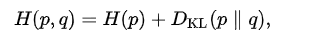
其中p(x)代表了真实分布,q(x)代表了预测分布
代码验证
import torch
import torch.nn as nn
import torch.nn.functional as F

# logits shape: [BS, NC]
batchsize = 2
num_class = 4

# 神经网络的输出值,没有经过softmax,未归一化
logits = torch.randn(batchsize, num_class)
# delta 目标分布
hard_label = torch.randint(num_class, size=(batchsize,))
# 非 delta 目标分布
soft_label = torch.randn(batchsize, num_class)


ce_loss_fn_sample = torch.nn.CrossEntropyLoss(reduction="none")
ce_loss_sample = ce_loss_fn_sample(logits, torch.softmax(soft_label, dim=-1))
print(f"cross entropy loss sample: {ce_loss_sample}")

kld_loss_fn_sample = torch.nn.KLDivLoss(reduction="none")
kld_loss_sample = kld_loss_fn_sample(torch.log(torch.softmax(logits, dim=-1)), torch.softmax(soft_label, dim=-1)).sum(-1)
print(f'Kullback-Leibler divergence loss sample:{kld_loss_sample}')

target_information_entropy = torch.distributions.Categorical(probs=torch.softmax(soft_label, dim=-1)).entropy()
print(f'information entropy sample:{target_information_entropy}')  # IE为常数,如果目标分布是delta分布,IE=0

print(torch.allclose(ce_loss_sample, kld_loss_sample+target_information_entropy))
对于delta分布,即对于onehot变量,信息熵是一个0,0对于卷积神经网络的参数更新时没有任何贡献的,此时,优化CE_loss与优化KLD_loss是没有任何区别,效果是一样的
对于非delta分布,即对于非onehot变量,信息熵是一个常数,常数对于卷积神经网络的参数更新时没有任何贡献的,此时,优化CE_loss与优化KLD_loss是没有任何区别,效果是一样的
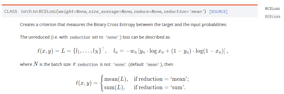
5.Binary Cross Entropy loss(BCE loss)
对判别器输出是真还是假,就属于二分类问题了
代码示例
import torch
import torch.nn as nn
import torch.nn.functional as F

# logits shape: [BS, 1]

bce_loss_fn = torch.nn.BCELoss()
nll_fn = torch.nn.NLLLoss()

batchsize = 2
logits = torch.randn(batchsize)
prob_1 = torch.sigmoid(logits)
target = torch.randint(2, size=(batchsize, ))
bce_loss = bce_loss_fn(prob_1, target.float())
print(f"binart cross entropy loss: {bce_loss}")

### 用NLL loss代替BCE loss做二分类
prob_0 = 1-prob_1.unsqueeze(-1)
prob = torch.cat([prob_0, prob_1.unsqueeze(-1)], dim=-1)
nll_loss_binary = nll_fn(torch.log(prob), target)
print(f"negative likelihood loss binary: {nll_loss_binary}")
print(torch.allclose(bce_loss, nll_loss_binary))
本质上,都是2个概率分布的映射
sigmoid 的作用是将输出值转换为0-1之间的浮点型
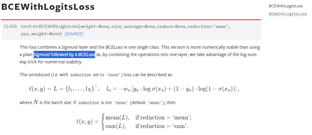
如果不想添加sigmoid函数的话,那么就直接用BCEWithLogitsLoss函数,如下图
但是,在BCE loss函数中,当输入数值变大的情况下,容易出现为0的情况,如下代码及结果所示:
import torch
import torch.nn as nn
import matplotlib.pyplot as plt
logits = torch.linspace(-10, 10, 2000)
loss = []
loss_fn = nn.BCELoss()
for lgs in logits:
    loss.append(loss_fn(torch.sigmoid(lgs), torch.ones_like(lgs)))
plt.plot(logits, loss)
plt.show()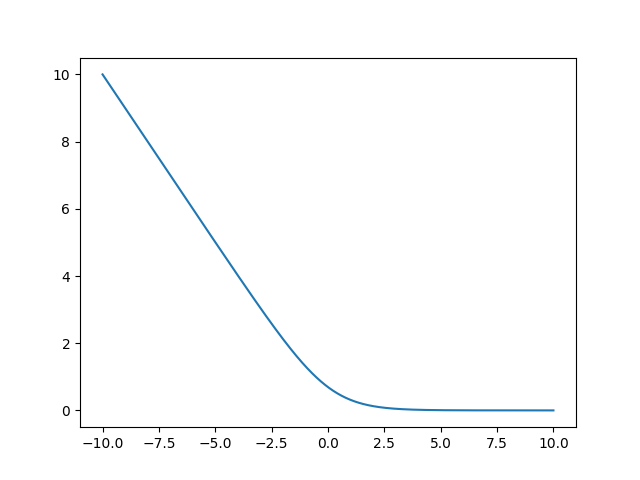
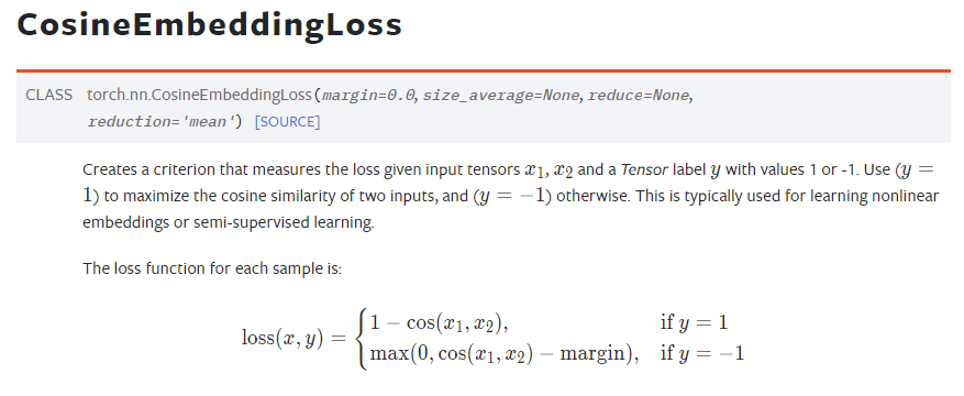
6.Cosine Similarity loss
数学表达式
import torch
import torch.nn as nn
import torch.nn.functional as F

batchsize = 2

cosine_loss_fn = torch.nn.CosineEmbeddingLoss()

#生成具有正态分布(均值为0,标准差为1)的随机数的函数
v1 = torch.randn(batchsize, 512)
v2 = torch.randn(batchsize, 512)
# target只能是0或者1
# 因此:0~1 -> 0~2 -> -1~1
target = torch.randint(2, size=(batchsize, ))*2-1
cosine_loss = cosine_loss_fn(v1, v2, target)
print(f"cosine similarity loss: {cosine_loss}")
应用领域
- 自监督学习
- 对比学习
- 相似度匹配
- 文本检索
- 图像检索
7.前述分类损失函数测试代码汇总
import torch
import torch.nn as nn
import torch.nn.functional as F

# logits shape: [BS, NC]
batchsize = 2
num_class = 4

logits = torch.randn(batchsize, num_class)
target_indices = torch.randint(num_class, size=(batchsize,))  # delta 目标分布
target_logits = torch.randn(batchsize, num_class)  # 非 delta 目标分布

# 1. 交叉熵损失 Cross Entropy Loss (CE loss)
print("----------------------------------------------------------")
## 1. 调用 Cross Entropy loss

### method 1 for CE loss
ce_loss_fun = torch.nn.CrossEntropyLoss()
ce_loss = ce_loss_fun(logits, target_indices)
print(f"cross entropy loss1: {ce_loss}")

### method 2 for CE loss
ce_loss = ce_loss_fun(logits, torch.softmax(target_logits, -1))
print(f"cross entropy loss2: {ce_loss}")

# 2.负对数似然损失 Negative Log Likelihood Loss (NLL loss)
print("----------------------------------------------------------")

nll_fn = torch.nn.NLLLoss()
nll_loss = nll_fn(torch.log(torch.softmax(logits, dim=-1)), target_indices)  # 与 CE loss结果相同
print(f"negative log-likelihood loss: {nll_loss}")
### cross entropy value = NLL value

# 3. 调用 Kullback-Leibler divergence loss(KL loss)
print("----------------------------------------------------------")

kld_loss_fn = torch.nn.KLDivLoss()
kld_loss = kld_loss_fn(torch.log(torch.softmax(logits, dim=-1)), torch.softmax(target_logits, dim=-1))
print(f'Kullback-Leibler divergence loss:{kld_loss}')

# 4.验证 CE = IE + KLD
print("----------------------------------------------------------")

ce_loss_fn_sample = torch.nn.CrossEntropyLoss(reduction="none")
ce_loss_sample = ce_loss_fn_sample(logits, torch.softmax(target_logits, dim=-1))
print(f"cross entropy loss sample: {ce_loss_sample}")

kld_loss_fn_sample = torch.nn.KLDivLoss(reduction="none")
kld_loss_sample = kld_loss_fn_sample(torch.log(torch.softmax(logits, dim=-1)), torch.softmax(target_logits, dim=-1)).sum(-1)
print(f'Kullback-Leibler divergence loss sample:{kld_loss_sample}')

target_information_entropy = torch.distributions.Categorical(probs=torch.softmax(target_logits, dim=-1)).entropy()
print(f'information entropy sample:{target_information_entropy}')  # IE为常数,如果目标分布是delta分布,IE=0

print(torch.allclose(ce_loss_sample, kld_loss_sample+target_information_entropy))

# 5.Binary Cross Entropy loss(BCE loss)
print("----------------------------------------------------------")

bce_loss_fn = torch.nn.BCELoss()
logits = torch.randn(batchsize)
prob_1 = torch.sigmoid(logits)
target = torch.randint(2, size=(batchsize, ))
bce_loss = bce_loss_fn(prob_1, target.float())
print(f"binart cross entropy loss: {bce_loss}")

### 用NLL loss代替BCE loss做二分类
prob_0 = 1-prob_1.unsqueeze(-1)
prob = torch.cat([prob_0, prob_1.unsqueeze(-1)], dim=-1)
nll_loss_binary = nll_fn(torch.log(prob), target)
print(f"negative likelihood loss binary: {nll_loss_binary}")
print(torch.allclose(bce_loss, nll_loss_binary))

# 6.调用 Cosine Similarity loss
print("----------------------------------------------------------")

cosine_loss_fn = torch.nn.CosineEmbeddingLoss()
v1 = torch.randn(batchsize, 512)
v2 = torch.randn(batchsize, 512)
target = torch.randint(2, size=(batchsize, ))*2-1
cosine_loss = cosine_loss_fn(v1, v2, target)
print(f"cosine similarity loss: {cosine_loss}")
运行结果
- 分类的损失函数,本质上是2个概率分布的比较
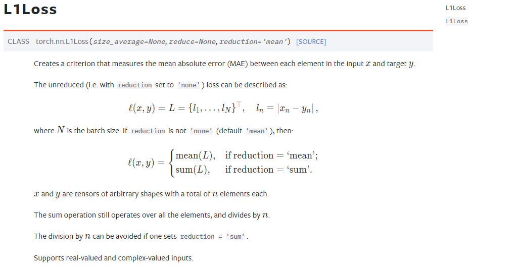
8.L1loss
- 也被成为MAE
- 基本不用在分类中
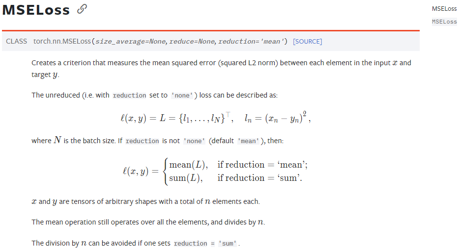
9.MSEloss
- 即为MSE
- 基本不用在分类中